Understand How Valves & Fittings Affect Head Loss

This series discusses valves and fittings and evaluates how these devices affect the operation of piping systems. Part 1 (Pumps & Systems, May 2015) covered head loss, K value and L/D coefficient. You can read part 1 here.

C_V Coefficient

The C_V value is an indication of the capacity of a valve or fitting and is often used to describe the performance of control valves. The C_V coefficient is often used to describe the hydraulic characteristics of elements in a pipeline. The definition of C_V is the number of U.S. gallons per minute (gpm) of 60 F water flowing through a valve or fitting results in a 1 pound per square inch (psi) pressure drop across the device.

For example, if a device has a C_V value of 200, then when 200 gpm flows through the device, a 1 psi pressure drop would occur. Equation 6 describes the C_V value.

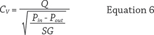
Where
C_V = Flow coefficient (unitless)
Q = Flow rate (gpm)
P = Pressure (psi)
SG = Specific gravity of the fluid (unitless)

The equation can be rearranged to allow for the solution of the flow rate for a given pressure drop and the pressure drop for a given flow rate.

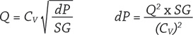
Equation 6 gives the result of using C_V in differential pressure instead of head. If a manufacturer provides information in C_V, users must convert it to differential pressure, then convert the results to head loss. Equation 7 can be used to eliminate the need to convert from pressure to head. It allows for the conversion of a C_V value to a K value.

Where
K = Resistance coefficient (unitless)
C_V = Flow coefficient (unitless)
d = internal diameter (inches)

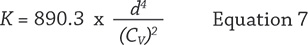
Calculating the Head Loss Using K Value

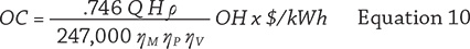
Regardless of the method used to arrive at a K value for a valve or fitting, Equation 8 is used to calculate the head loss resulting from valves and fittings.

When multiple valves and fittings in a pipeline have the same diameter, the K values for each valve or fitting can be added. The sum of the K values can be used to calculate the head loss for all the valves and fittings.

To demonstrate, calculate the head loss for the valves and fittings in a pipeline when 600 gpm of water is flowing through the following valves and fittings: a sharp-edged transition from a tank to pipeline, a full-seated globe valve and a strainer with a C_V value of 450. These full-seated devices are in a 6-inch pipe with a turbulent friction factor of 0.015 inches. The K values are listed in Table 1. The resulting head loss with 600 gpm going through the pipeline is shown in Equation 9.

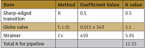Table 1. Calculation of K value for different methods describing valves and fittings (Graphics courtesy of the author)

Cross Section of Valves & Fittings

Reference 1 has cross sections of types of valves and fittings and the corresponding K values or L/D coefficients. There are too many types of valves and fittings to present in this article, but some attributes can be generalized. For example, a full-seat ball valve with its straight-through design has a much lower L/D value than a globe valve through which the fluid must make four changes of direction and flow around the valve disk within the flow path. The type of valve employed is based on many factors. Leak tightness is an important factor, but when two types of valves meet the same requirements, it is recommended to use the one with the lower head loss.

Another example of fittings with varied loss coefficients are elbows. A short radius 90-degree elbow has an L/D coefficient of 20, but a long radius 90-degree elbow has a L/D coefficient of 14. This may not seem like a significant loss, but it adds up. So do the associated costs. The pump must supply the energy that is lost across the valves and fitting.

Cost of Pipeline Operation

To demonstrate the pumping cost associated with valves and fittings, calculate the operating costs for different types of valves and fittings. Equation 10 can determine the pumping cost.

Where
OC = Operating cost ($/time)
Q = Flow rate (gpm)
H = Head (feet of fluid)
ρ = Density (lb/ft3)
η = Efficiency, M motor, P pump, V variable speed drive (VSD) (percent)
O = Operating hours in evaluation (hours)
$/kWh = Electrical power cost ($/kWh)

In this example, the pump efficiency is 70 percent, and the motor efficiency is 90 percent. No VSD is installed, the evaluation period is 8,000 hours, and the cost of power is $0.10/kilowatt-hour (kWh). This example evaluates 4-inch valves and fittings with a flow rate of 400 gpm. The results are presented in Table 2.

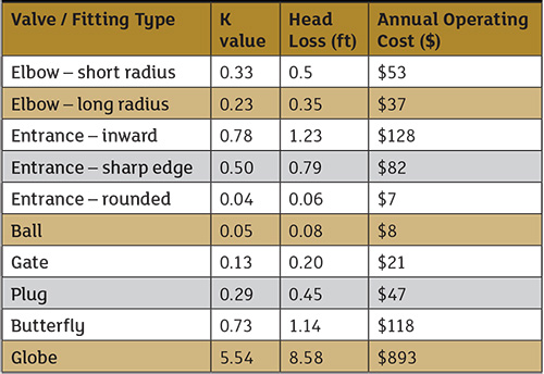Table 2. The relationship between K values, head loss and annual operating cost for valves and fittings. The example is for 4-inch valves and fittings passing 400 gpm.

Every item placed in a piping system has an operating cost. This should be considered every time a user specifies a valve time or adds elbows.

Conclusion

The often overlooked performance of the multitude of valves and fittings adds up. They have a compounded effect on performance in a fluid operation and need to be taken into consideration for efficiency planning and optimization.

Next month's column will investigate how the control elements operate and the role that these devices play in piping systems and their associated cost.